MPU6050

How to use MPU6050 as an IMU sensor

Overview

Please check my older post for review on Orientation representation

1. MPU6050 Overview & Configuration

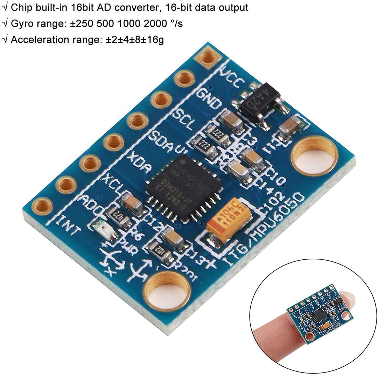
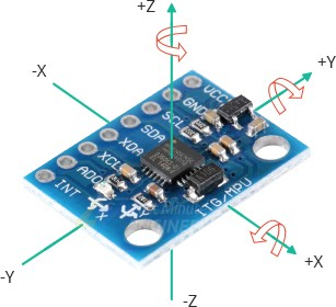
Documentation:

MPU6050 Initialization Steps

Initialize $I^2C$ Address:
Default address is usually 0x68 (or 0x69 if AD0 is HIGH).
Set Power Management (PWR_MGMT_1):
Wake up the MPU6050 from sleep mode.
Write SLEEP bit on PWR_MGMT_1 register (0x6B) to 0.
Set Digital Low-Pass Filter (DLPF):
Configure DLPF_CFG bits on CONFIG register (0x1A) for signal smoothing.
Set sampling rate:
Configure SMPLRT_DIV register (0x19) for the sample rate.
Set Sensitivity Ranges:
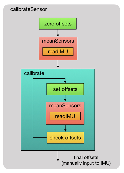
Write to GYRO_CONFIG register (0x1B) and ACCEL_CONFIG register (0x1C).
Set Calibration Offsets:
Write to OFFSET registers.

Digital Low Pass Filter (DLPF) Configuration (`DLPF_CONFIG`)

To set the bandwidth rate of the accelerometer and the gyroscope, configure the DLPF_CFG bits (bits 0~2) in the CONFIG register.

Register	Name
`0x1A`	`CONFIG`

DLPF_CFG	Acc BW (Hz)	Acc Delay (ms)	Acc Fs (kHz)	Gyro BW (Hz)	Gyro Delay (ms)	Gyro Fs (kHz)
`0`	260	0	1	256	0.98	8
`1`	184	2.0	1	188	1.9	1
`2`	94	3.0	1	98	2.8	1
`3`	44	4.9	1	42	4.8	1
`4`	21	8.5	1	20	8.3	1
`5`	10	13.8	1	10	13.4	1
`6`	5	19.0	1	5	18.6	1
`7`	Reserved	Reserved	1	Reserved	Reserved	8

Notes

Question: Why don’t we always use high bandwidth data?

Reasons:

High-Frequency Noise Exposure
The raw gyroscope and accelerometer readings will fluctuate wildly, making it impossible to see the actual orientation of the device.
Microcontroller and Battery Strain
High bandwidth demands faster sensor output rates (up to 8 kHz).
The microcontroller must spend a massive amount of CPU cycles processing thousands of data points per second.

Sampling rate

To set the sampling rate of the sensor, configure the DLPF_CFG bits (bits 0~2) in the CONFIG register.

Register	Name
`0x19`	`SMPLRT_DIV`

\[\text{Sample Rate} = \frac{\text{Gyroscope Fs}}{1 + \text{SMPLRT_DIV}}\]

Note: only applicable if DLPF is enabled (DLPF_CFG is 1~6).

Gyroscope Configuration (`GYRO_CONFIG`)

To set the full-scale range of the gyroscope, configure the FS_SEL bits (bits 3 and 4) in the GYRO_CONFIG register.

Register	Name
`0x1B`	`GYRO_CONFIG`

FS_SEL	Full Scale Range	LSB Sensitivity
`0`	$\pm 250^\circ/\text{s}$	$131\text{ LSB}/(^\circ/\text{s})$
`1`	$\pm 500^\circ/\text{s}$	$65.5\text{ LSB}/(^\circ/\text{s})$
`2`	$\pm 1000^\circ/\text{s}$	$32.8\text{ LSB}/(^\circ/\text{s})$
`3`	$\pm 2000^\circ/\text{s}$	$16.4\text{ LSB}/(^\circ/\text{s})$

Accelerometer Configuration (`ACCEL_CONFIG`)

To set the full-scale range of the accelerometer, configure the AFS_SEL bits (bits 4 and 5) in the ACCEL_CONFIG register.

Register	Name
`0x1C`	`ACCEL_CONFIG`

AFS_SEL	Full Scale Range	LSB Sensitivity
`0`	$\pm 2\text{ g}$	$16384\text{ LSB/g}$
`1`	$\pm 4\text{ g}$	$8192\text{ LSB/g}$
`2`	$\pm 8\text{ g}$	$4096\text{ LSB/g}$
`3`	$\pm 16\text{ g}$	$2048\text{ LSB/g}$

Calibration flow

2. Orientation Estimation

The sensor provides raw data reading from accelerometer and gyroscope. However, in pratical, what we need is an orientation estimation based on this data.

Data processing is required to estimate the orientation based on these two sensors. There are several processing methods, here are few notable processing method to get orientation from MPU6050.

Kalman Filter
Kalman filter is an algorithm to estimate the state of a system with uncertainty.
This algorithm is mathematically optimal on linear systems. However, it requires more tuning and computation load to handle matrices.
Complementary Filter
Complementary filter acts as the alternative of Kalman Filter.
Internal DMP (Digital Motion Processing)
Internal Digital Motion Processing™ (DMP™) engine supports 3D MotionProcessing and gesture recognition algorithms.

	Kalman Filter	Complementary Filter	Internal DMP
How it Works	Uses a statistical physics model to dynamically weight sensor trust based on variance.	High-pass filters the gyroscope; low-pass filters the accelerometer. Blends them with a simple fixed ratio (e.g., 98/2).	MPU6050’s internal hardware coprocessor calculates orientation entirely off the main MCU.
Setup & Tuning Complexity	Difficult Requires tuning multiple process and measurement noise covariance matrices (Q and R).	Very Easy. Adjust one alpha tuning parameter (e.g., α = 0.98).	Moderate. Requires utilizing specific library code (like the Jeff Rowberg I2Cdevlib) to upload the firmware blob.
MCU Load	Moderate to High	Extremely Low (<1% on an Arduino UNO)	Near Zero
Output Data Types	Euler angles or Quaternions.	Euler angles (Roll, Pitch).	Quaternions, Euler angles, Yaw/Pitch/Roll, and Gravity vectors.

This note will explains further about complementary filter.

Complementary Filter

The complementary filter is a simple sensor fusion algorithm.

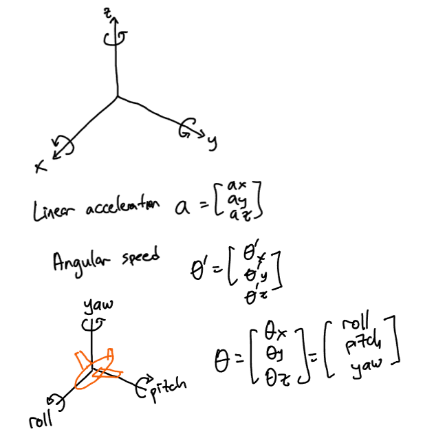
Getting orientation may simply be obtained by integrating the angular velocity $\theta’$ over time, theoretically. However, on real sensors, integrating means repeatedly adding up increments of small systematic errors. This phenomenon causes gyroscopic drift, which causes the gyroscope data becomes inaccurate on a longer run.

Getting orientation is also possible from the acceleration of the rigid body, since there is always gravitational acceleration applied on the body. However, this calculation becomes inaccurate when other accelerations are applied on the body. Therefore, the orientation from accelerometer may not be accurate on a short run affected by noise or perturbations.

The complementary filter “fuses” the gyroscope data and the accelerometer data to cancel the errors from each method. The idea is to apply high-pass filter on the gyroscope data –to cancel the long-term error– and low-pass filter on the accelerometer data –to cancel the short-term error–.

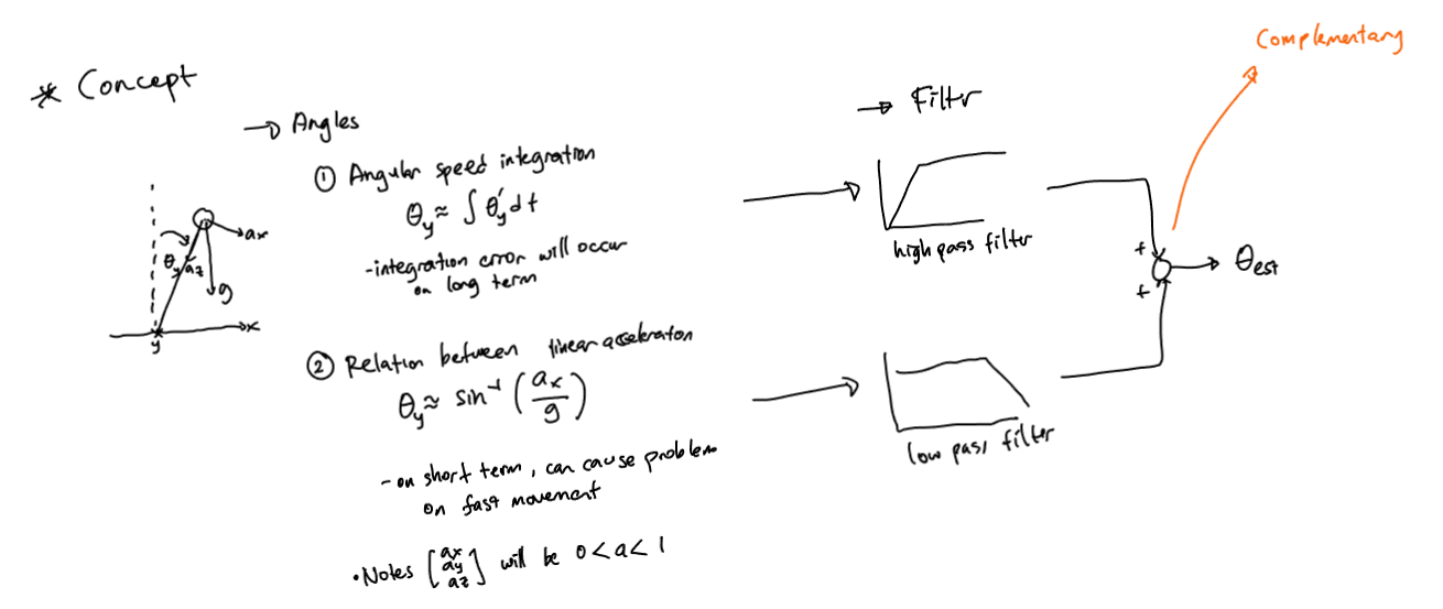
Complementary Filter Equations

The Complementary Filter combines high-frequency gyroscope integration with low-frequency accelerometer angle estimations to eliminate gyroscope drift and high-frequency accelerometer noise:

\[\theta_{\text{filtered}} = \alpha \cdot \theta_{\text{gyro}} + (1 - \alpha) \cdot \theta_{\text{accel}}\] \[\theta_{\text{filtered}} = \alpha \cdot (\theta_{\text{prev}} + \omega \cdot \Delta t) + (1 - \alpha) \cdot \theta_{\text{accel}}\]

$\alpha = \frac{T}{T + dt} $, where $T$ : Time constant, and $dt$ : Sampling rate
$\alpha$ : High-pass filter coefficient for gyroscope integration. Typically $\approx 0.96 \sim 0.98$.
$(1 - \alpha)$ : Low-pass filter coefficient for accelerometer output

More details on the equation

From frequency domain perspective, a High-pass filter (HPF) transfer function:

\[H_{HPF}(s) = \frac{s}{s+\omega_o}\]

, and a Low-pass filter (LPF) transfer function:

\[H_{LPF}(s) = \frac{\omega_o}{s+\omega_o}\]

where $\omega_o = \frac{1}{RC}$.

The complementary filter in Laplace domain:

\[\Theta (s) = H_{gyro}(s) \cdot \Theta_{gyro}(s) + H_{accel}(s) \cdot \Theta_{accel}(s)\] \[\Theta (s) = \frac{s}{s+\omega_o} \cdot \Theta_{gyro}(s) + \frac{\omega_o}{s+\omega_o} \cdot \Theta_{accel}(s)\] \[\Theta (s) = \frac{s}{s+\omega_o} \cdot \Theta_{gyro}(s) + (1 - \frac{s}{s+\omega_o}) \cdot \Theta_{accel}(s)\] \[\Theta (s) = \alpha \cdot \Theta_{gyro}(s) + (1 - \alpha) \cdot \Theta_{accel}(s)\]

Roll and Pitch from Accelerometer

Using gravity acceleration components ($a_x, a_y, a_z$) measured by the accelerometer:

\[\theta_{x} = \tan^{-1}\left( \frac{a_y}{\sqrt{a_x^2 + a_z^2}} \right)\] \[\theta_{y} = \tan^{-1}\left( \frac{a_x}{\sqrt{a_y^2 + a_z^2}} \right)\]

Note: Yaw ($\theta_{z}$) cannot be derived accurately using an accelerometer alone because gravity acts vertically along the $z$-axis.